This guide covers both basic and advanced usage of DistanceTransforms.jl.
Getting Started
Installation
usingPkgPkg.add("DistanceTransforms")
Basic Usage
The primary function in DistanceTransforms.jl is transform. This function processes an array of 0s and 1s, converting each background element (0) into a value representing its squared Euclidean distance to the nearest foreground element (1).
usingImages# Download and load example imageimg =load(download("http://docs.opencv.org/3.1.0/water_coins.jpg"))# Convert to binary imageimg_bw =Gray.(img) .>0.5# Apply distance transformimg_tfm =transform(boolean_indicator(img_bw))# Visualizefig =Figure(size = (900, 300))ax1 =Axis(fig[1, 1], title ="Original Image")ax2 =Axis(fig[1, 2], title ="Segmented Image")ax3 =Axis(fig[1, 3], title ="Distance Transform")heatmap!(ax1, rotr90(img), colormap =:grays)heatmap!(ax2, rotr90(img_bw), colormap =:grays)heatmap!(ax3, rotr90(img_tfm), colormap =:grays)hidedecorations!.([ax1, ax2, ax3])fig
Understanding Euclidean Distance
The library, by default, returns the squared Euclidean distance. If you need the true Euclidean distance, you can take the square root of each element:
usingImageMorphology: distance_transform, feature_transform# Apply ImageMorphology distance transformeuc_transform2 =distance_transform(feature_transform(Bool.(array2)))# Compare resultsprintln("Are the results approximately equal?")isapprox(euc_transform2, euc_transform; rtol =1e-2)
Are the results approximately equal?
true
Advanced Features
Multi-threading
DistanceTransforms.jl efficiently utilizes multi-threading, particularly in its Felzenszwalb distance transform algorithm.
⚠️ Julia might only load with 1 thread which makes the actual benchmark below meaningless and potentially confusing. Use this for understanding how to use the threaded kwarg ⚠️
Number of threads: 1
Single-threaded minimum time: 17.508084 ms
Multi-threaded minimum time: 17.558 ms
Speedup factor: 0.9971570793940084
GPU Acceleration
DistanceTransforms.jl extends its performance capabilities with GPU acceleration. The library uses Julia’s multiple dispatch to automatically leverage GPU resources when available.
CUDA Example
usingCUDAusingDistanceTransforms# Create a random array on GPUx_gpu = CUDA.rand([0, 1], 1000, 1000)x_gpu =boolean_indicator(x_gpu)# The transform function automatically uses GPUresult_gpu =transform(x_gpu)# Transfer result back to CPU if neededresult_cpu =Array(result_gpu)
Metal Example
usingMetalusingDistanceTransforms# Create a random array on GPUx_gpu = Metal.rand([0, 1], 1000, 1000)x_gpu =boolean_indicator(x_gpu)# The transform function automatically uses GPUresult_gpu =transform(x_gpu)# Transfer result back to CPU if neededresult_cpu =Array(result_gpu)
Performance Benchmarks
Performance comparison across different implementations for 2D and 3D distance transforms:
Performance Comparison
As shown in the graph, the GPU implementation demonstrates superior performance, especially for larger arrays.
Best Practices
For small arrays (<100x100): CPU with multi-threading is often sufficient
For medium arrays: Multi-threaded CPU may be faster than GPU due to lower overhead
For large arrays (>1000x1000): GPU acceleration provides the best performance
For 3D data: GPU acceleration is strongly recommended due to the computational complexity
Algorithm Details
On the CPU, DistanceTransforms.jl uses the squared Euclidean distance transform algorithm by Felzenszwalb and Huttenlocher, known for its accuracy and efficiency. On the GPU, thanks to the amazing AcceleratedKernels.jl and KernelAbstraction.jl packages, the algorithm is essentially identical.
Source Code
---title: "User Guide"sidebar: juliaformat: html: toc: trueexecute: engine: julia julia: threads: 4---This guide covers both basic and advanced usage of DistanceTransforms.jl.## Getting Started### Installation```juliausing PkgPkg.add("DistanceTransforms")```### Basic UsageThe primary function in DistanceTransforms.jl is `transform`. This function processes an array of 0s and 1s, converting each background element (0) into a value representing its squared Euclidean distance to the nearest foreground element (1).```{julia}using DistanceTransforms: transform, boolean_indicatorusing CairoMakie: Figure, Axis, heatmap!, hidedecorations!# Create a random binary arrayarr = rand([0, 1], 10, 10)# Apply distance transformtransformed = transform(boolean_indicator(arr))# Create visualizationfig = Figure(size = (800, 400))ax1 = Axis(fig[1, 1], title = "Original")ax2 = Axis(fig[1, 2], title = "Distance Transform")heatmap!(ax1, arr, colormap = :grays)heatmap!(ax2, transformed, colormap = :grays)fig```### Real-World ExampleLet's apply a distance transform to a real image:```{julia}using Images# Download and load example imageimg = load(download("http://docs.opencv.org/3.1.0/water_coins.jpg"))# Convert to binary imageimg_bw = Gray.(img) .> 0.5# Apply distance transformimg_tfm = transform(boolean_indicator(img_bw))# Visualizefig = Figure(size = (900, 300))ax1 = Axis(fig[1, 1], title = "Original Image")ax2 = Axis(fig[1, 2], title = "Segmented Image")ax3 = Axis(fig[1, 3], title = "Distance Transform")heatmap!(ax1, rotr90(img), colormap = :grays)heatmap!(ax2, rotr90(img_bw), colormap = :grays)heatmap!(ax3, rotr90(img_tfm), colormap = :grays)hidedecorations!.([ax1, ax2, ax3])fig```### Understanding Euclidean DistanceThe library, by default, returns the squared Euclidean distance. If you need the true Euclidean distance, you can take the square root of each element:```{julia}# Create sample binary arrayarray2 = [ 0 1 1 0 1 0 0 0 1 0 1 1 0 0 0]# Convert to boolean indicatorarray2_bool = boolean_indicator(array2)# Apply squared Euclidean distance transformsq_euc_transform = transform(array2_bool)# Convert to true Euclidean distanceeuc_transform = sqrt.(sq_euc_transform)# Display resultsprintln("Squared Euclidean Distance: $(sq_euc_transform)")println("Euclidean Distance: $(euc_transform)")```### Comparison with ImageMorphology.jl```{julia}using ImageMorphology: distance_transform, feature_transform# Apply ImageMorphology distance transformeuc_transform2 = distance_transform(feature_transform(Bool.(array2)))# Compare resultsprintln("Are the results approximately equal?")isapprox(euc_transform2, euc_transform; rtol = 1e-2)```## Advanced Features### Multi-threadingDistanceTransforms.jl efficiently utilizes multi-threading, particularly in its Felzenszwalb distance transform algorithm.⚠️ Julia might only load with `1 thread` which makes the actual benchmark below meaningless and potentially confusing. Use this for understanding how to use the `threaded` kwarg ⚠️```{julia}using BenchmarkToolsusing Base.Threads: nthreads# Create a random binary arrayx = boolean_indicator(rand([0, 1], 1000, 1000))# Single-threaded benchmarksingle_threaded = @benchmark transform($x; threaded = false)# Multi-threaded benchmarkmulti_threaded = @benchmark transform($x; threaded = true)# Display resultsprintln("Number of threads: $(nthreads())")println("Single-threaded minimum time: $(minimum(single_threaded).time / 1e6) ms")println("Multi-threaded minimum time: $(minimum(multi_threaded).time / 1e6) ms")println("Speedup factor: $(minimum(single_threaded).time / minimum(multi_threaded).time)")```### GPU AccelerationDistanceTransforms.jl extends its performance capabilities with GPU acceleration. The library uses Julia's multiple dispatch to automatically leverage GPU resources when available.#### CUDA Example```juliausing CUDAusing DistanceTransforms# Create a random array on GPUx_gpu = CUDA.rand([0, 1], 1000, 1000)x_gpu = boolean_indicator(x_gpu)# The transform function automatically uses GPUresult_gpu = transform(x_gpu)# Transfer result back to CPU if neededresult_cpu = Array(result_gpu)```#### Metal Example```juliausing Metalusing DistanceTransforms# Create a random array on GPUx_gpu = Metal.rand([0, 1], 1000, 1000)x_gpu = boolean_indicator(x_gpu)# The transform function automatically uses GPUresult_gpu = transform(x_gpu)# Transfer result back to CPU if neededresult_cpu = Array(result_gpu)```### Performance BenchmarksPerformance comparison across different implementations for 2D and 3D distance transforms: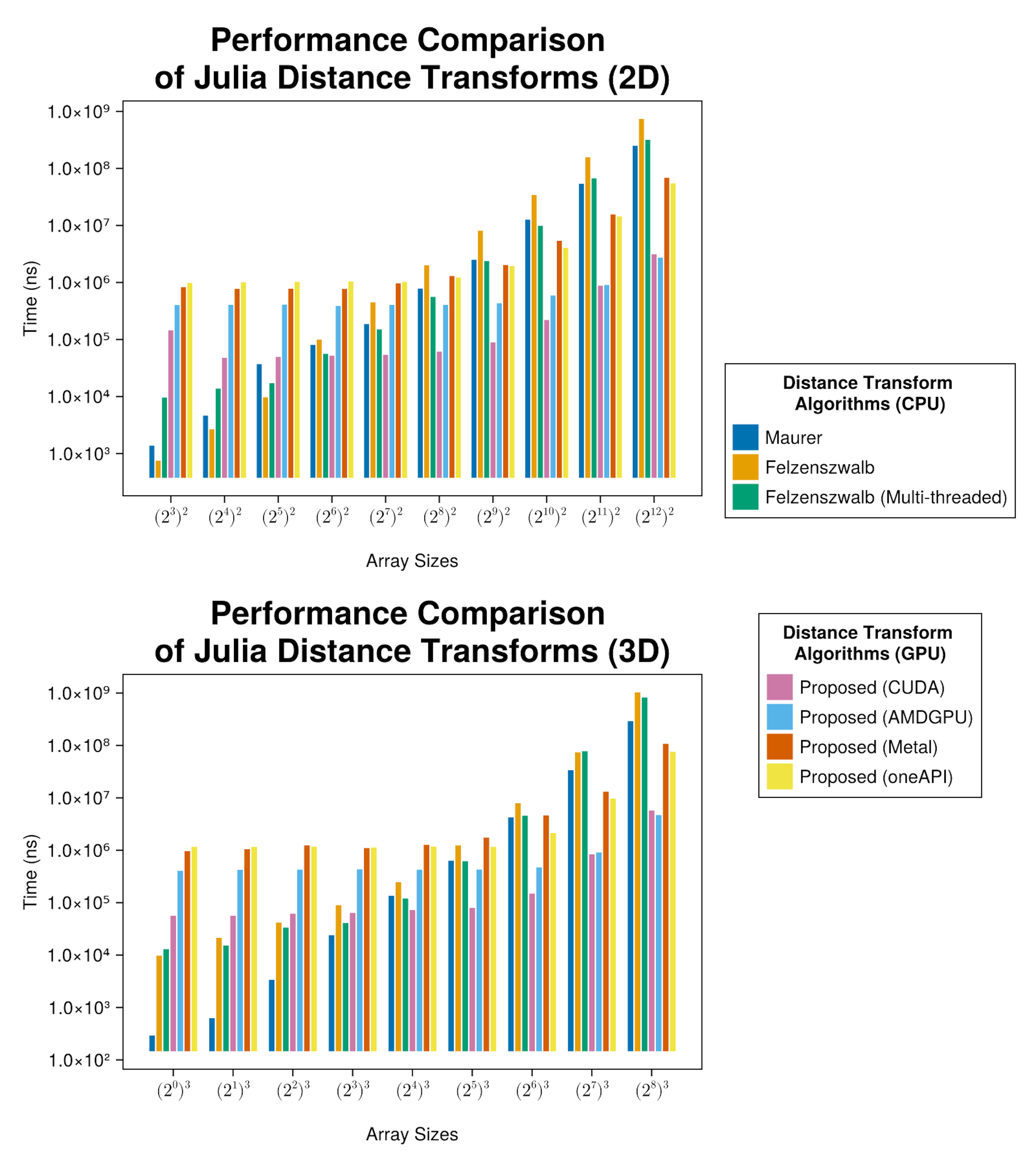As shown in the graph, the GPU implementation demonstrates superior performance, especially for larger arrays.### Best Practices1. **For small arrays (<100x100)**: CPU with multi-threading is often sufficient2. **For medium arrays**: Multi-threaded CPU may be faster than GPU due to lower overhead3. **For large arrays (>1000x1000)**: GPU acceleration provides the best performance4. **For 3D data**: GPU acceleration is strongly recommended due to the computational complexity## Algorithm DetailsOn the CPU, DistanceTransforms.jl uses the squared Euclidean distance transform algorithm by [Felzenszwalb and Huttenlocher](https://theoryofcomputing.org/articles/v008a019/), known for its accuracy and efficiency. On the GPU, thanks to the amazing [AcceleratedKernels.jl](https://github.com/JuliaGPU/AcceleratedKernels.jl) and [KernelAbstraction.jl](https://github.com/JuliaGPU/KernelAbstractions.jl) packages, the algorithm is essentially identical.

